A Geodesic Cut-Cell Prior for Neural Skinning

Abstract

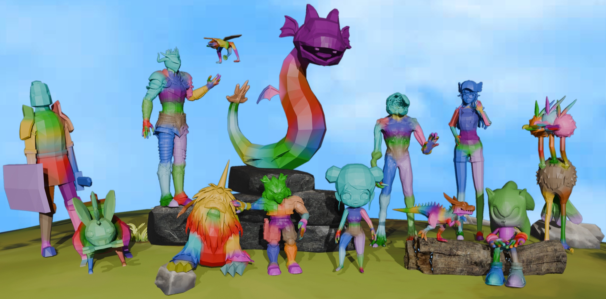
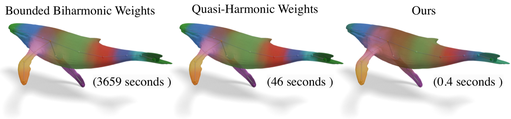
We introduce cut-cell skinning, a geometric prior designed to augment data-driven skinning weight generation. While data-driven methods show promise in producing high-quality skinning weights, they often lack the generalizability of classic geometric approaches. To bridge this gap, we propose a geometric prior that can be robustly computed for in-the-wild meshes and is efficient for large-scale machine learning workflows. The key idea of our cut-cell skinning is a fast graph-based approximation of the volumetric geodesics distances, motivated by their importance in classic skinning weight computation. Our method achieves orders of magnitude speedup compared to optimization-based solvers and remains resilient to topological artifacts common in cage- or voxel-based alternatives. We demonstrate the efficacy of the cut-cell skinning prior by integrating it into recent neural skinning models, showing consistent improvements across existing methods and achieving state-of-the-art results.

Video

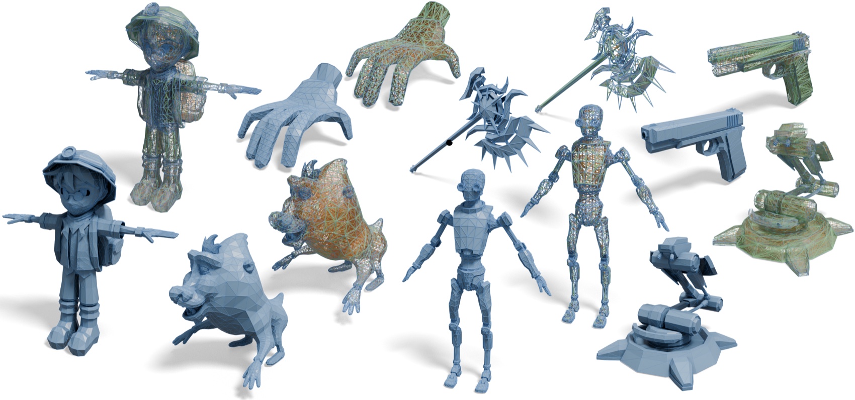
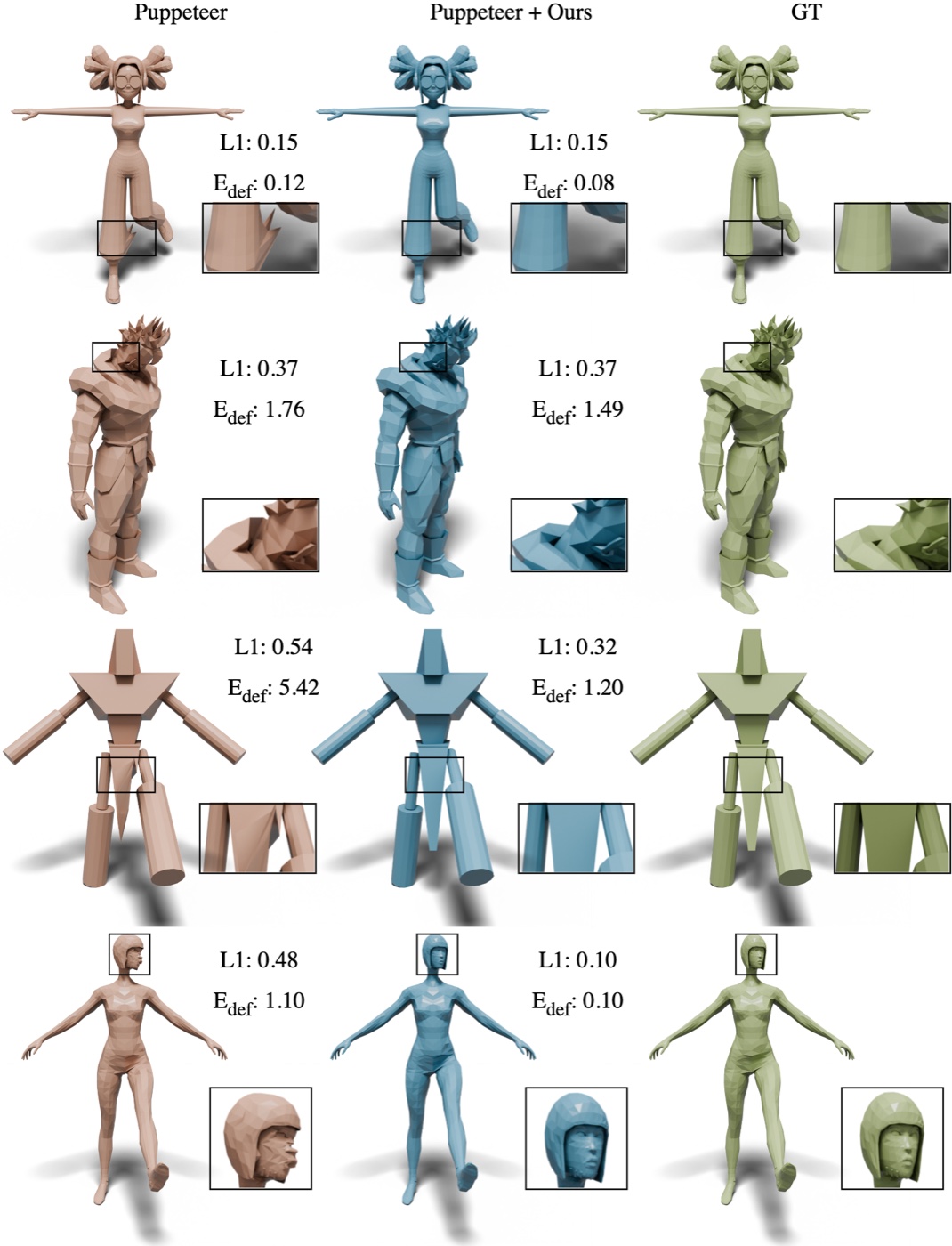
Each clip plays one motion three ways: the baseline, the same model augmented with our cut-cell prior, and the artist-authored ground truth, annotated with their L1 and deformation errors. Comparisons cover Puppeteer, UniRig, and RigNet.

Method

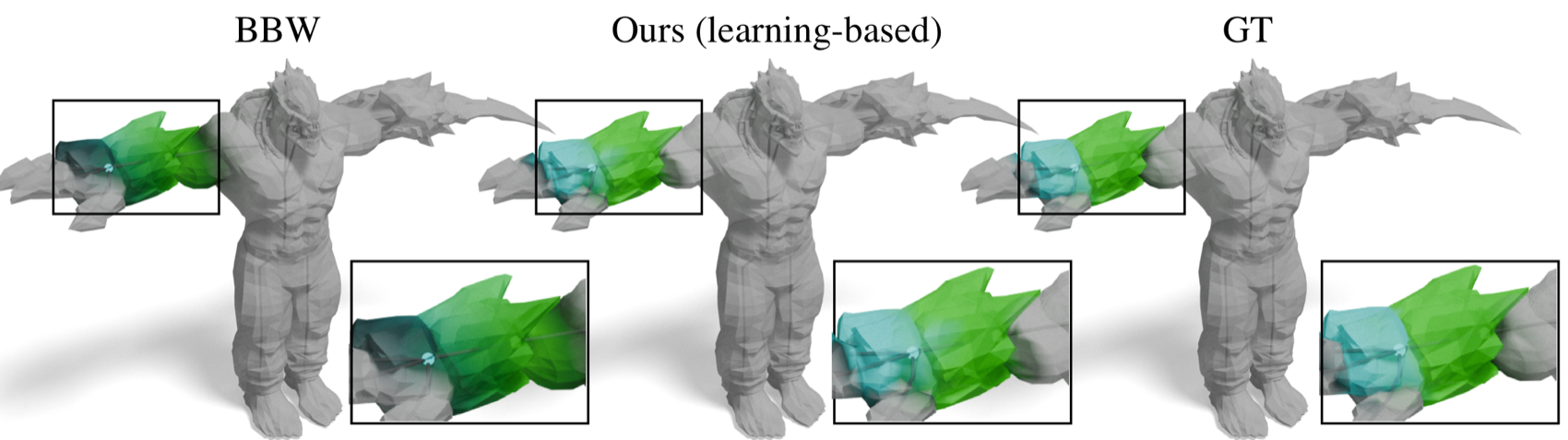
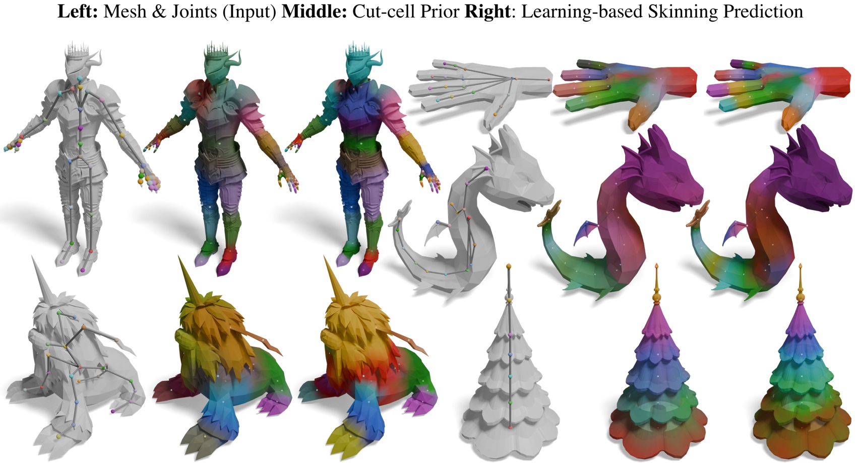
Automated geometric methods compute skinning weights by solving constrained optimization problems. They generalize well, but often fail to capture the semantic nuances required to articulate characters with material heterogeneity. Machine learning alternatives capture those semantics, yet struggle to generalize. Can a geometric method instead be integrated as an inductive bias that guides data-driven inference?

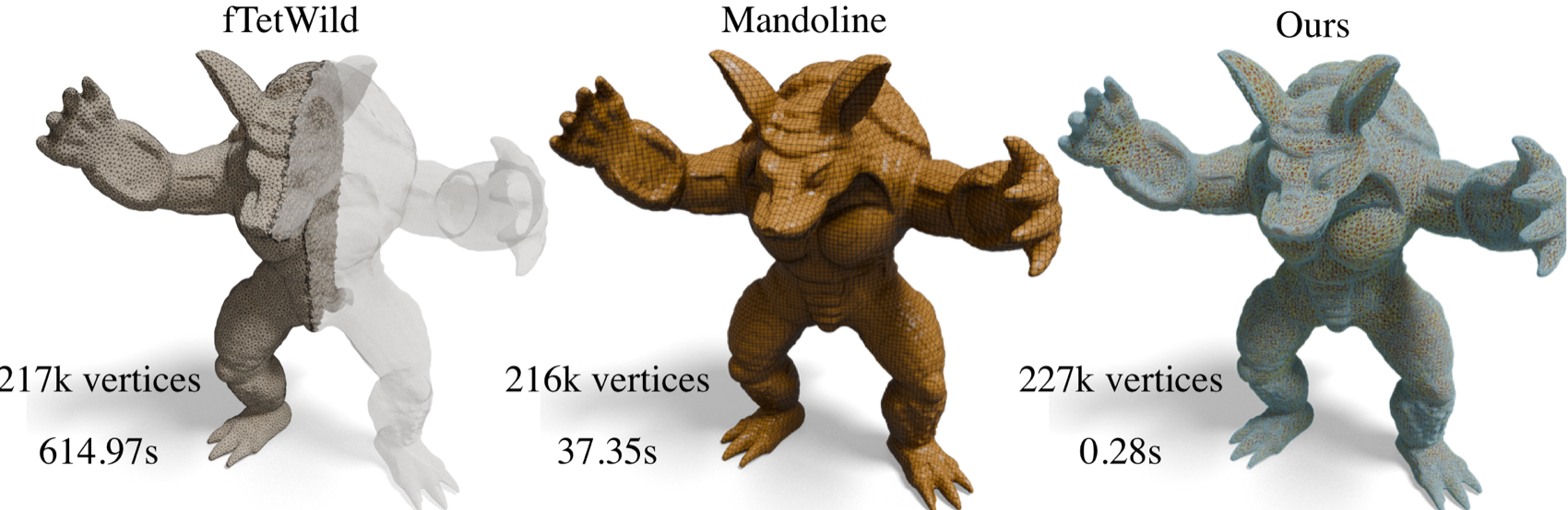
Three copies of a muscular creature with a rocky forearm. Bounded biharmonic weights bleed across the rock boundary, our result matches the crisp boundary of the ground truth. — Artist-created weights respect the semantics of the geometry, such as the rocky lower arm. Pure geometric methods (left) have no semantic awareness. Our approach (middle) combines data-driven learning with a robust geometric prior.

Geometric methods are also expensive. Volumetric meshing and optimization-based solvers take minutes to hours per mesh, which is intractable for large-scale datasets.

Three volumetric discretizations of the same character: a tetrahedral mesh from fTetWild, a cut-cell mesh from Mandoline, and our cut-cell graph. — Tetrahedral meshes (fTetWild, left) and cut-cell meshes (Mandoline, middle) are high-quality volumetric representations, but their construction cost makes them impractical for large-scale datasets.

Three weight visualizations of the same creature labeled bounded biharmonic weights at 3659 seconds, quasi-harmonic weights at 46 seconds, and ours at 0.4 seconds. — Runtime for skinning prior computation, excluding meshing and graph construction. Optimization-based methods are challenging to operate on large scale datasets.

Versus voxels and cages

Voxel-based approximations such as Geodesic Voxel Binding are robust to imperfect geometry, but merge parts that are spatially close yet geodesically distant. Cage-based coordinates suffer the same failure, and additionally require watertight cages with correct topology.

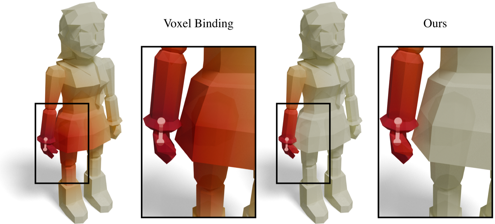
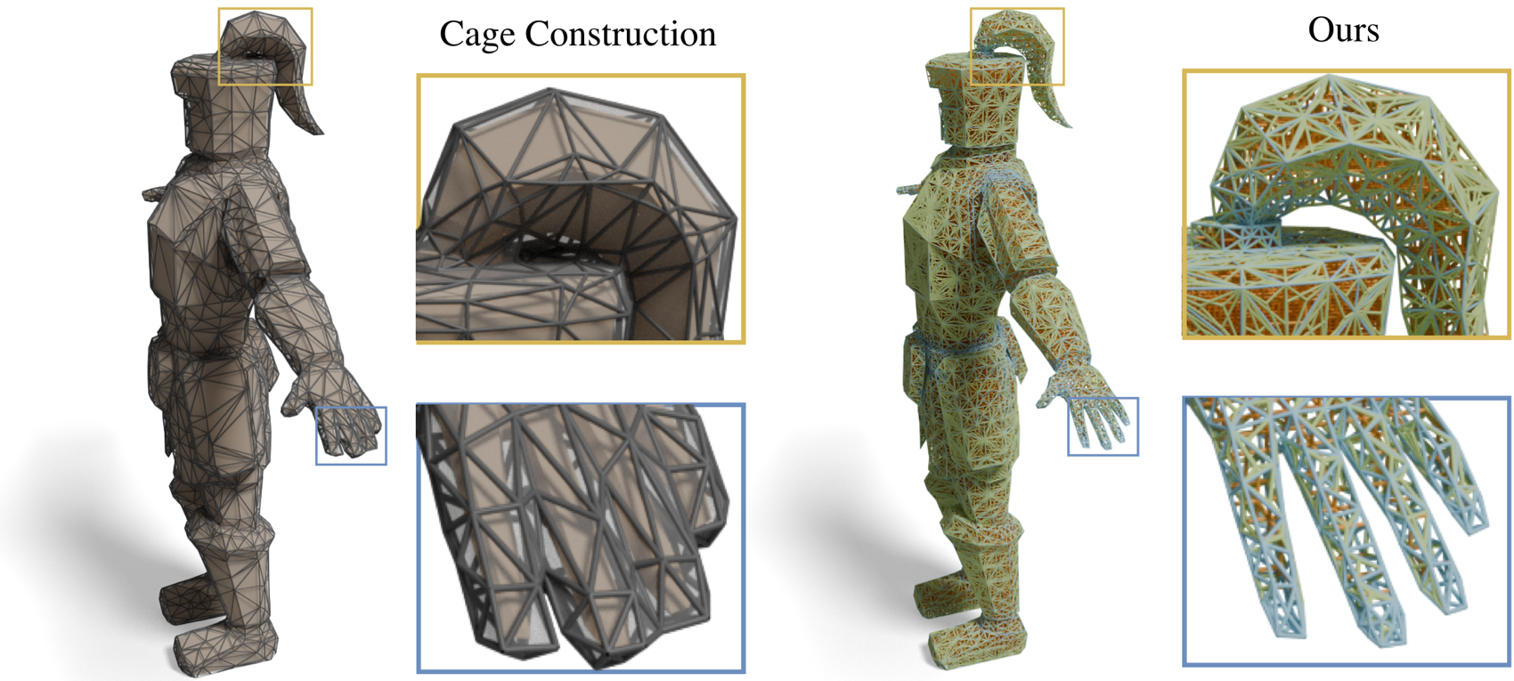
Distance fields on a character with a hand resting near the torso. The voxelized method leaks distance across the gap, the cut-cell result keeps hand and torso distinct. — Voxelization introduces unintended connections across narrow gaps, such as the hand and the torso.

Cut-cell graph

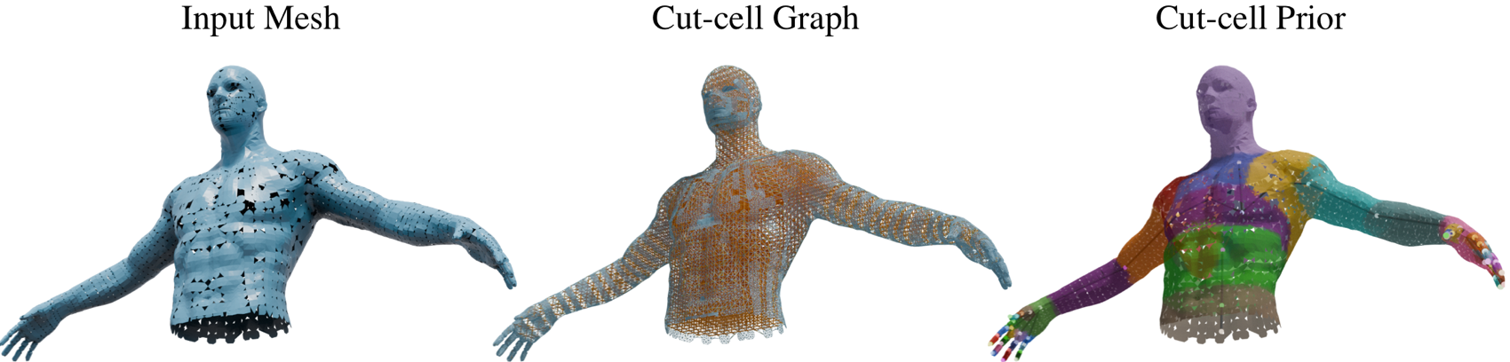
We propose an efficient alternative — the Cut-Cell Graph — to approximate the true volumetric geodesic distances with graph geodesics at a substantially lower computational cost. Our graph construction “cuts” through grid cells with the input surface, thus inheriting the terminology “cut-cell” from fluid simulation.

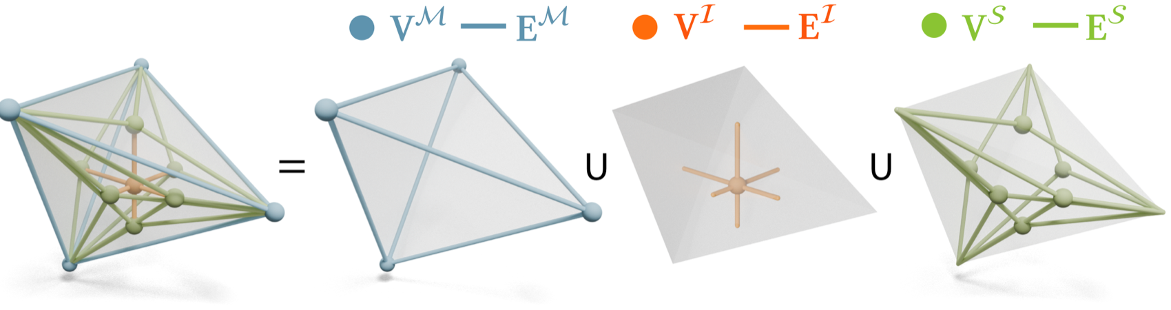
A tetrahedron-like shape whose graph is decomposed into three overlaid parts: blue mesh vertices and edges, orange interior grid vertices and edges, and green surface intersection vertices and edges. — A cut-cell graph G consists of vertices V^M and edges E^M from the input mesh, interior vertices V^I and edges E^I from the voxel grid, and surface vertices V^S where the mesh and the grid meet. Edges E^S connect V^S to V^M so that all graph vertices are connected.

Construction involves only two extremely robust subroutines, both trivially parallelizable:

Ray casting. With the mesh pre-normalized to the unit cube, cast axis-aligned rays along each of the three directions. Grid vertices and mesh intersections cut every ray into candidate segments.
Generalized winding number. Query it at each segment midpoint to classify inside from outside, and keep the interior segments together with their vertices.

Each surface intersection is then connected to the three corner vertices of the triangle it hits, and the original mesh vertices and edges are added to the graph.

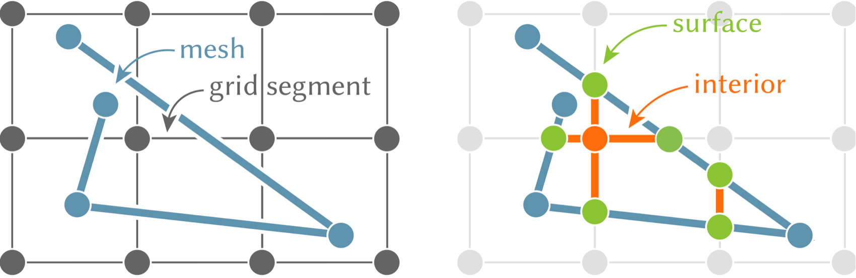
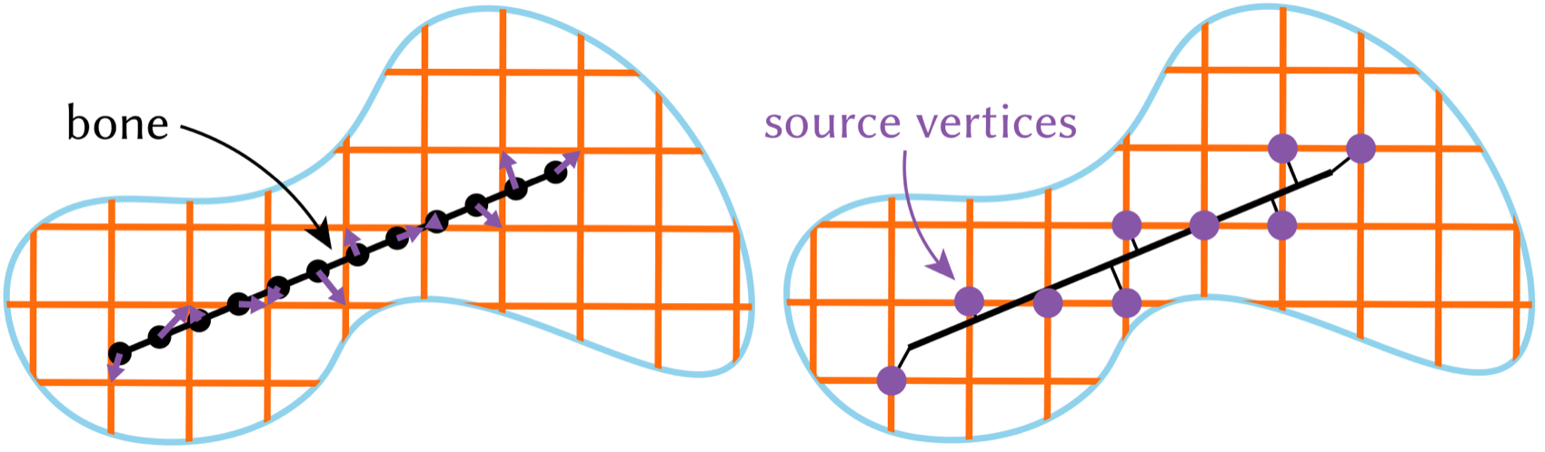
A ray passing through a 2D shape, split by black grid vertices and blue surface crossings into segments, with interior segments highlighted in orange. — For each grid segment, diced by the grid vertices (black) and the mesh (blue), we use the *generalized winding number* to decide whether they lie on the interior of the mesh. If they are, we keep their edges (orange) and tip vertices (green and orange).

Gallery pairing in-the-wild input meshes with their cut-cell graphs, drawn as dense orange interior edges, green surface crossings, and blue mesh wireframe. — Cut-cell graphs (right) for in-the-wild input meshes (left). Orange denotes the *interior*, green the *surface intersection*, and blue the input *mesh*.

To turn the graph into a skinning prior, we sample N = 5 points on each bone and take their closest graph vertices as sources. Dijkstra’s algorithm then yields the shortest graph geodesic distance d_ij from every vertex i to every bone j.

Diagram showing points sampled along a bone, purple arrows pointing to their nearest graph vertices, and the resulting set of purple source vertices used to seed Dijkstra's algorithm. — Points sampled on the bone (black, left) “vote” for their closest graph vertices. The resulting source vertices (purple, right) seed the distance traversal.

A kernel maps these distances to skinning weights, which are rescaled at each vertex for partition of unity. Here α controls smoothness and D is the bounding box extent:

w_ij=(1(1 − α) (d_ij/D) + α (d_ij/D)²)²

Gallery of characters shown three ways: input mesh with joints, the cut-cell skinning prior, and the neural prediction built on that prior, both weight visualizations using rainbow per-joint colors. — Paired input meshes and joints, the cut-cell skinning prior, and neural skinning predictions based on the prior.

Speed

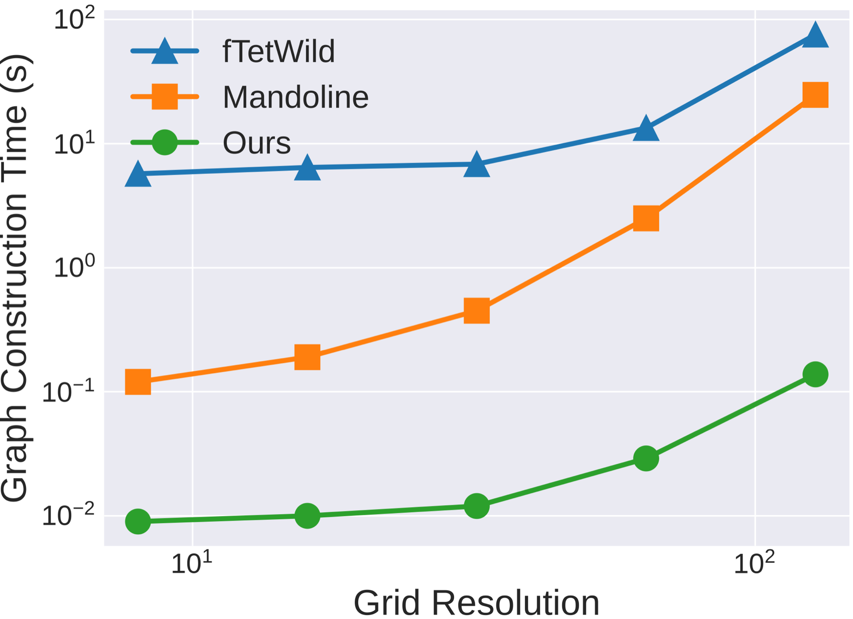
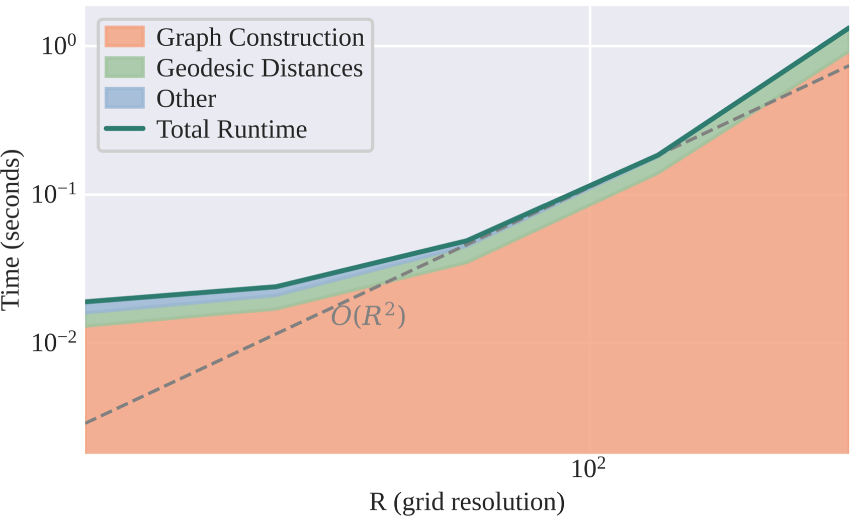
Even a baseline CPU implementation of our approach achieves orders-of-magnitude speedups over alternative volumetric meshing techniques.

Graph construction time in seconds. Parentheses indicate our speedup over each baseline.

Grid resolution	8	16	32	64	128
fTetWild	5.72 636×	6.43 643×	6.84 570×	13.37 461×	75.58 548×
Mandoline	0.12 13×	0.19 19×	0.45 38×	2.50 86×	24.69 179×
Ours	0.009	0.010	0.012	0.029	0.138

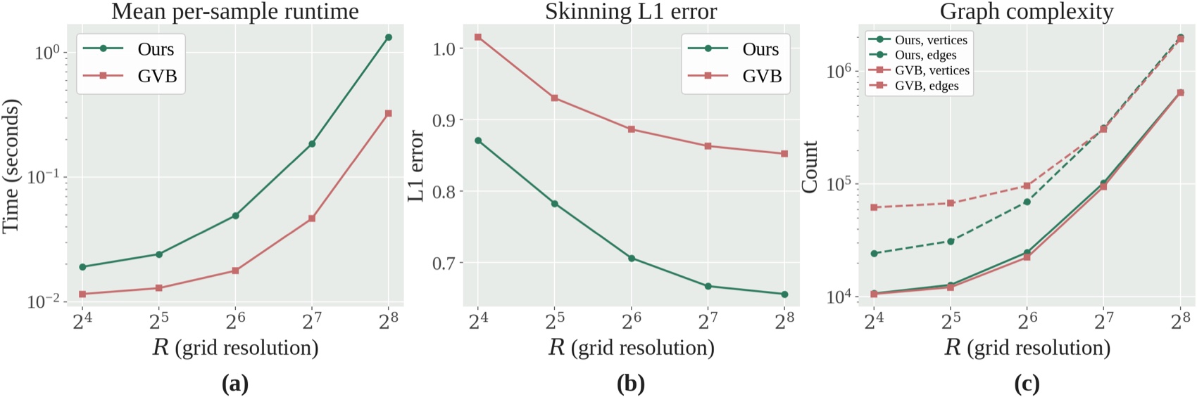
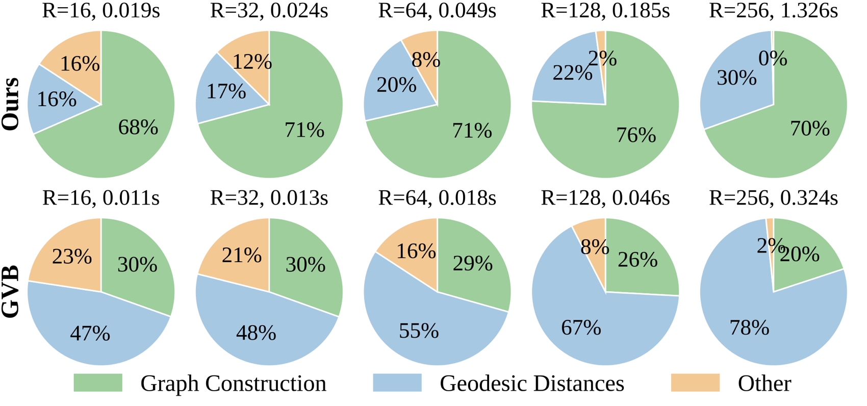
Log-log plot of graph construction time versus grid resolution. Our curve sits two to three orders of magnitude below fTetWild and Mandoline at every resolution. — Graph construction time vs. grid resolution.

Stacked area plot of total prior computation time against grid resolution, split into graph construction, geodesic distances, and other, tracking an O of R squared reference line. — Total prior computation time vs. grid resolution.

Against Geodesic Voxel Binding, our prior is more accurate at every resolution, and reaches higher accuracy at a much coarser grid (R = 64 vs. R = 256).

Three plots against grid resolution: runtime, skinning L1 error, and graph complexity, comparing ours to geodesic voxel binding. — Runtime, L1 error, and graph complexity compared with Geodesic Voxel Binding.

Two rows of pie charts across grid resolutions showing that graph construction dominates our runtime while geodesic distance computation dominates geodesic voxel binding. — Runtime breakdown of the cut-cell prior and geodesic voxel binding, where R denotes the grid resolution.

Results

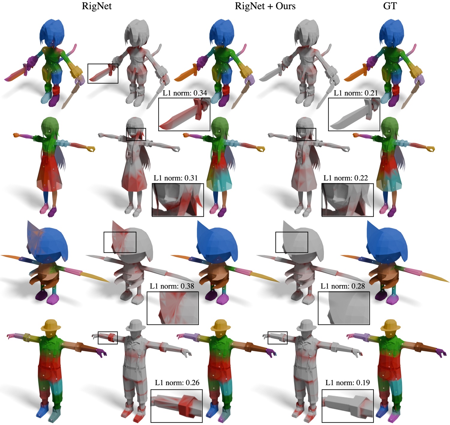
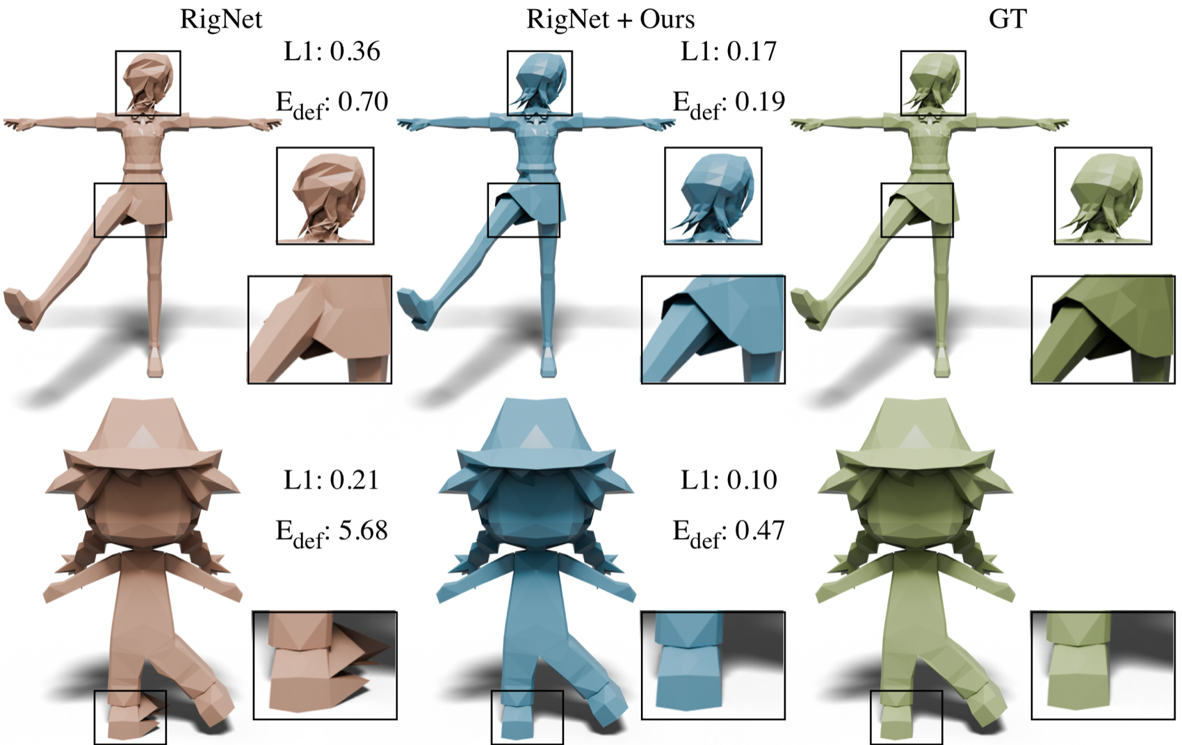
We replace RigNet’s voxel-based geodesic distances with graph geodesic distances computed on our cut-cell graph. Evaluated on ModelsResource.

Method	avg L1 ↓	Precision ↑	Recall ↑	E_def ↓
RigNet	0.432	0.803	0.794	8.58
RigNet + Ours	0.367	0.850	0.798	6.06
Improvement	15.05%	5.85%	0.50%	29.37%

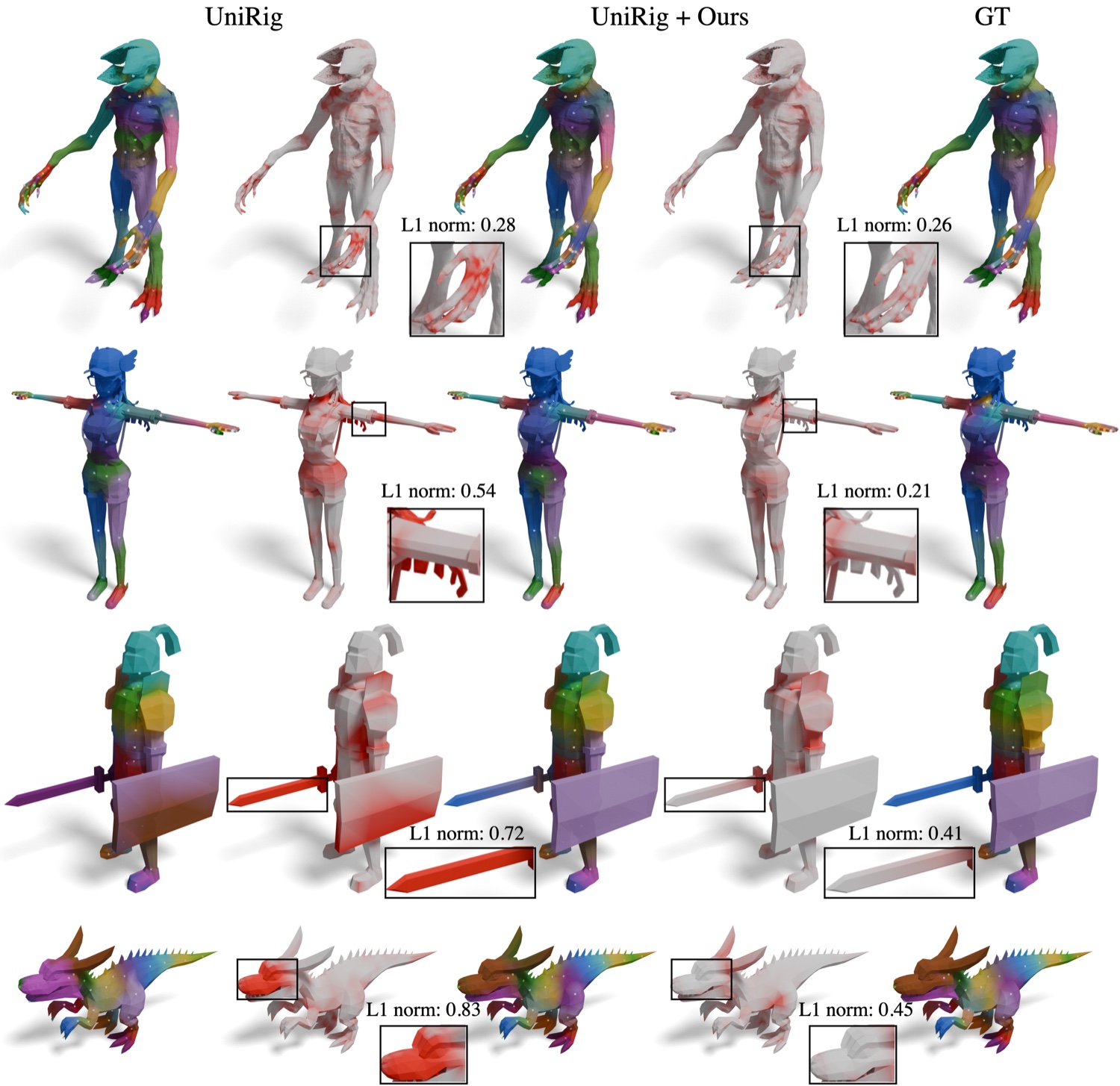
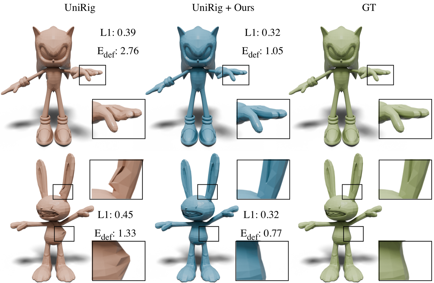
Qualitative skinning weight comparison on RigNet across several characters, with baseline, ours, and ground truth columns. — Our prior better separates geodesically distant but spatially close parts, such as long hair against the shoulder (second row).

Animated poses comparing RigNet against RigNet plus our prior, with red circles marking sticking artifacts at hair and feet in the baseline. — Under animation, the baseline produces visible “sticking” artifacts at the hair and feet.

We substitute our prior for UniRig’s voxel-based skinning weights, and the network is trained to predict the residual between the prior and the ground truth.

Method	Articulation-XL 2.0				Articulation-XL 2.0 (de-duplicated)
Method	avg L1 ↓	Prec. ↑	Recall ↑	E_def ↓	avg L1 ↓	Prec. ↑	Recall ↑	E_def ↓
UniRig	0.747	0.746	0.673	21.25	0.768	0.736	0.663	25.29
UniRig + Ours	0.386	0.820	0.850	10.91	0.447	0.794	0.829	14.18
Improvement	48.33%	9.92%	26.30%	48.66%	41.80%	7.88%	25.04%	43.93%

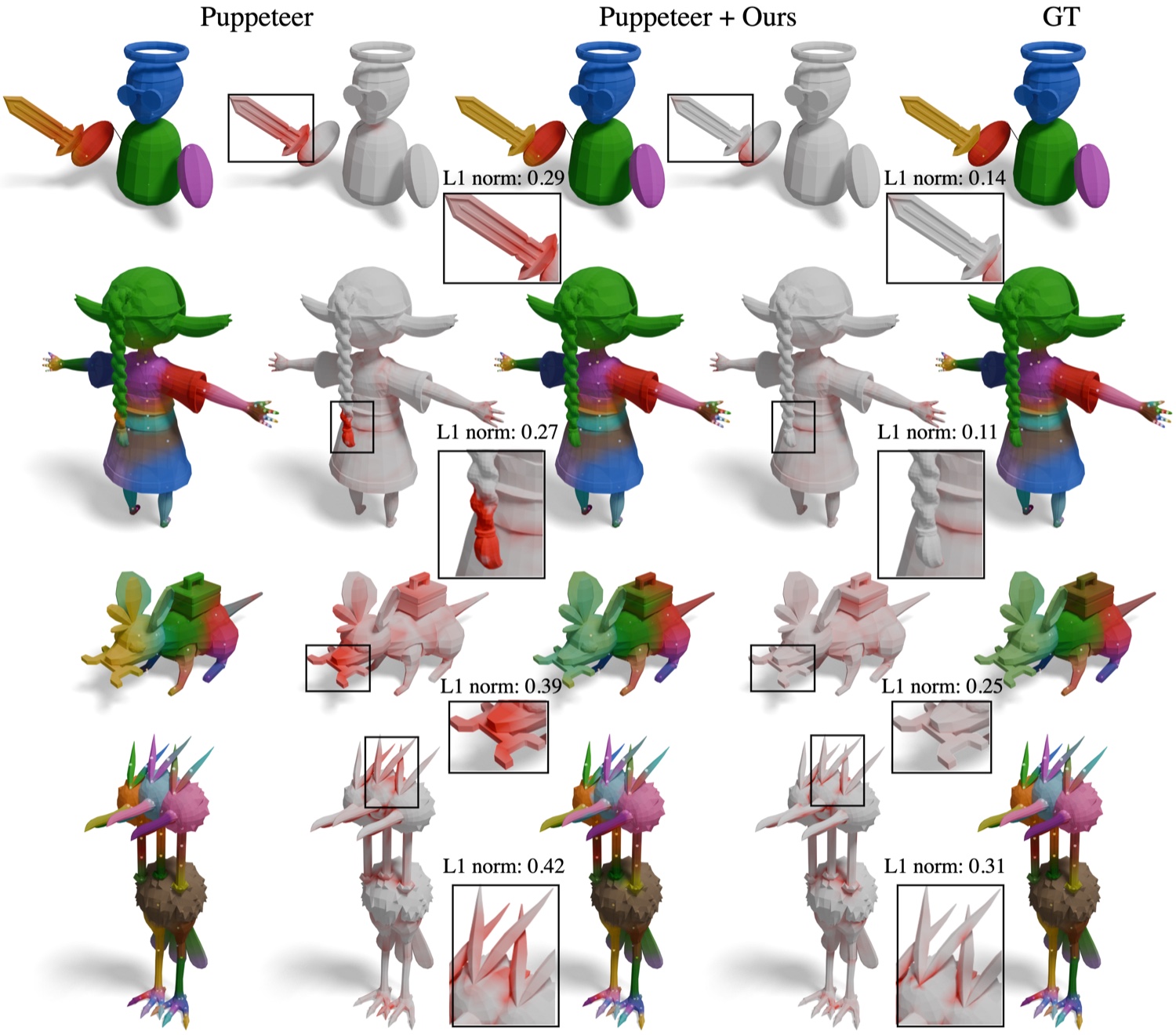
Qualitative skinning weight comparison on UniRig across several creatures, with baseline, ours, and ground truth columns. — Our prior helps the baseline disambiguate fine parts that lie spatially close yet are topologically far apart, such as the creature’s long claws (first row).

Animated poses comparing UniRig against UniRig plus our prior, showing a dragged middle finger and kinked rabbit ear in the baseline. — The baseline deforms slender extremities unnaturally: the middle finger is dragged along with the index finger, and the rabbit’s ear root and hip kink.

We concatenate the cut-cell weights with Puppeteer’s point features after the attention modules, and a lightweight MLP fuses them before the final similarity computation.

Method	Articulation-XL 2.0				Articulation-XL 2.0 (de-duplicated)
Method	avg L1 ↓	Prec. ↑	Recall ↑	E_def ↓	avg L1 ↓	Prec. ↑	Recall ↑	E_def ↓
Puppeteer	0.335	0.876	0.740	5.949	0.377	0.859	0.735	7.763
Puppeteer + Ours	0.320	0.896	0.724	5.333	0.368	0.877	0.712	7.453
Improvement	+4.48%	+2.28%	−2.16%	+10.36%	+2.39%	+2.10%	−3.13%	+3.99%

Qualitative skinning weight comparison on Puppeteer, including a character holding a sword whose weights leak from unrelated joints in the baseline. — On rare attached objects such as the sword (top row), the baseline leaks skinning weights from unrelated joints.

Four rows of animated comparisons against Puppeteer, annotated with L1 and deformation error values under each pose. — In the first two rows, both methods have nearly identical L1, yet our prior yields visibly cleaner deformations and a much lower E_def.

Robustness

Because the graph is built from fast winding number queries and axis-aligned ray casts, it is robust to non-watertight meshes, noisy geometry, and polygon soups.

An open, hole-riddled input mesh, the cut-cell graph built on it, and the resulting part-consistent skinning prior. — The input mesh (left) is open and non-watertight, with holes scattered across the surface. Our graph (middle) is still built robustly, and the resulting prior (right) yields part-consistent regions.

Acknowledgements

We thank the authors of RigNet, UniRig, and Puppeteer for releasing their code and pretrained checkpoints, which made the integrations and comparisons in this work possible.

BibTeX

@article{ma2026cutcell,
  title   = {A Geodesic Cut-Cell Prior for Neural Skinning},
  author  = {Ma, Wenchao and Dwarakanath, Surya and Ben-Shabat, Yizhak
             and Kneub{\"u}hler, Dario and Jiang, Haomiao
             and Huang, Sharon X. and Liu, Hsueh-Ti Derek},
  year    = {2026}
}

A Geodesic Cut-Cell Priorfor Neural Skinning